A balun at the centre of a dipole: what the NanoVNA proved, and what it did not

The antenna from the previous note — two legs of twisted pair, about twenty metres each, six metres up — worked beautifully on receive. What did not work was the place where the wire meets the cable. To begin with there was a twisted joint and insulating tape: a solution that lasts until the first rain and does not hold electrically at all.

On 8 December 2023 I built a proper centre: a balun on a ferrite toroid inside a sealed box. And, more to the point of this note, I checked it with an analyser — and then worked out that I had checked something other than what I thought.

Why a dipole needs a balun

A dipole is balanced: two identical legs about the feed point. Coax is unbalanced: the centre conductor and the braid are not equals. Join one straight to the other, and part of the current that should have gone into the second leg flows instead down the outside of the braid towards the rig.

The cable becomes a third leg of the antenna. On transmit that means a distorted pattern and an SWR that changes when you move the cable. On receive — and a receiver is what I had then — the consequence is nastier: the braid picks up whatever it passes. Switch-mode power supplies, LED lamps, chargers — everything that makes noise in the house lands on the cable and walks into the receiver alongside the wanted signal.

In my case that was not marginal theory. The wire hangs six metres up — not “well away from the house” but directly above it, in the same field of noise. There was nowhere to move the antenna to, so the least I could do was stop the noise taking a second route in, along the cable.

A 1:1 balun breaks that path: it passes the differential current, which is what the whole thing was built for, and opposes the common-mode current, the one that flows on the braid.

What that toroid turned out to be

The markings on the toroid itself cannot be read: it is wrapped first in white tape and then, all together, in black. Unwrapping proved unnecessary — the markings turned up somewhere else, in a purchase history: an M2000NM K32×20×9 ferrite toroid and PETD2-200 enamelled copper wire, 1.0 mm.

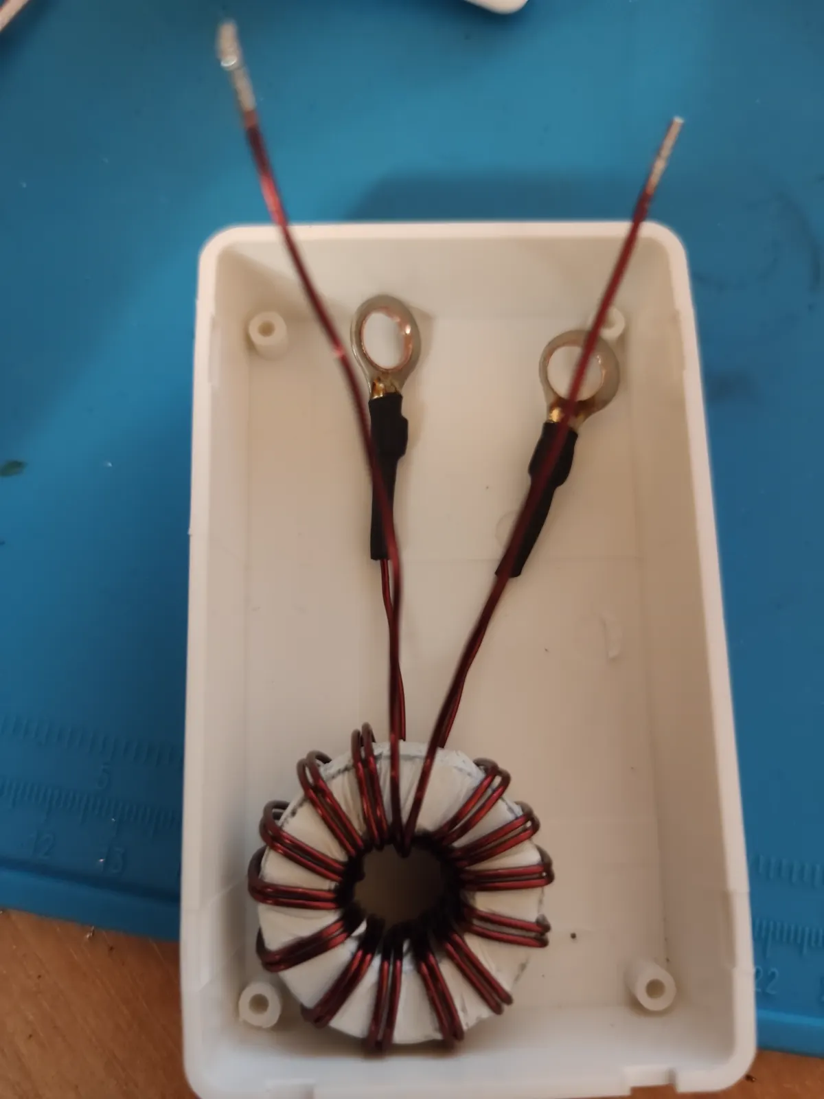
Size. K32×20×9 reads straightforwardly: 32 mm outside, 20 inside, 9 high. My estimate from the ruler in the photograph — “about 35–36 mm” — was three or four millimetres too generous: the winding and the tape add more to the overall size than the eye credits. In Western terms the core sits between an FT-114 (29.0 mm) and an FT-140 (35.6 mm).

Material. M2000NM is a manganese-zinc ferrite with an initial permeability of 2000. The closest Western equivalent is Fair-Rite 77: the same MnZn, the same μ_i = 2000. The guess — “a high-permeability ferrite, not powdered iron” — turned out right, and the core is exactly the class you would choose for this job deliberately.

The winding: 14 bifilar turns. Each turn is two wires laid side by side — the classic Guanella arrangement, where the two conductors form a length of transmission line on a shared core. The numbers agree with the photograph: 14 turns of a pair means 28 passes through the window, a millimetre and a bit each with the enamel, about 30 mm in all against an inner perimeter under the tape of roughly 56 mm. One layer with gaps — exactly what the close-up shows.

The white tape under the winding is not decoration, and it now has two reasons. The first is obvious: a ferrite toroid has sharp edges, and they cut the enamel where the wire bends over the rim. The second arrived with the markings: manganese-zinc ferrite is electrically conductive, its resistivity orders of magnitude lower than nickel-zinc. Laying bare wire straight onto a core like that is not a good idea, even with the enamel intact.

What that gives. The core constant comes from the geometry: mean magnetic path length l_e = π·(32 + 20)/2 ≈ 81.7 mm, cross-section A_e = 9·(32 − 20)/2 = 54 mm², hence A_L = μ₀·μ_i·A_e/l_e ≈ 1.66 µH/turn². On 14 turns that is 0.33 mH — but only if the permeability held at 2000. It does not: in MnZn ferrite μ′ starts falling above a megahertz while the losses rise. For a choke that is no misfortune but the working regime: the impedance simply stops being inductive and becomes resistive. Substituting the complex permeability of mix 77 — which is how the common-mode choke calculator works it out — 14 turns on this core give:

Band	Resistive part	Reactive part	Magnitude
160 m (1.84 MHz)	2.4 kΩ	+2.2 kΩ	3.3 kΩ
80 m (3.65 MHz)	3.6 kΩ	+1.3 kΩ	3.9 kΩ
40 m (7.1 MHz)	3.8 kΩ	≈ 0	3.8 kΩ
20 m (14.2 MHz)	3.2 kΩ	−0.6 kΩ	3.3 kΩ
15 m (21.2 MHz)	2.9 kΩ	−0.7 kΩ	3.0 kΩ
10 m (28.5 MHz)	2.7 kΩ	−0.8 kΩ	2.8 kΩ

So from 160 down to 10 metres it is three or four kilohms, and from forty metres upwards almost purely resistive. The “few kilohms” benchmark mentioned below is met — though without much margin. And this is a calculation from an equivalent material's data, not a measurement; why that wording stands as final will become clear.

Will it take transmit power. The very losses that make M2000NM a good choke turn into heat on transmit: common-mode current warms this core, and high-permeability MnZn is more vulnerable in that respect than nickel-zinc mixes 43 or 31. In December 2023 the question did not arise — a receiver was connected to the box. But later my first digital contacts went out through this same assembly, so the core did work on transmit, and in a mode where the carrier is held for the whole transmission. It survived. I would still not repeat that blind at a hundred watts: a core for that kind of power gets calculated afresh.

The box

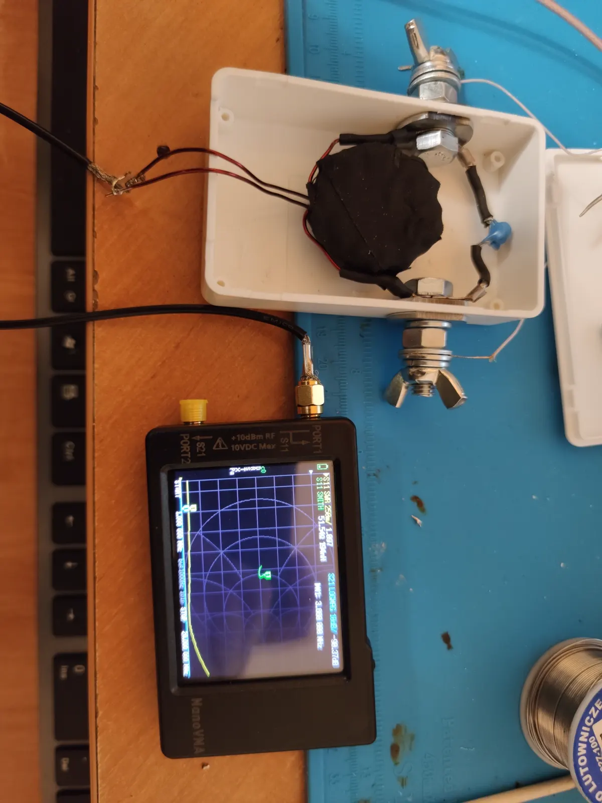
The enclosure is an ordinary junction box. Through-bolts with washers and wing nuts pass through opposite walls: the antenna legs fasten to them, and they can be tightened in winter wearing gloves, with no soldering iron up the mast. The toroid lies flat, wrapped in black tape. One joint is made with a blue crimp terminal, the rest are under heatshrink.

That is the standard of work one need not be ashamed of, and at the same time the standard that can be reached in an evening out of what is in the drawer.

The measurement

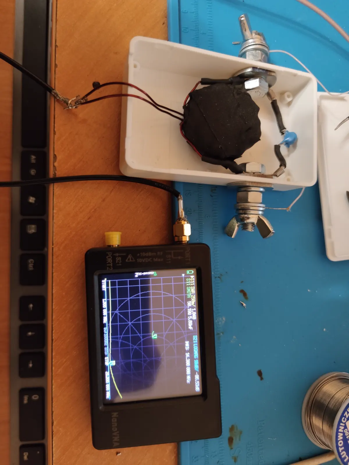
A NanoVNA, sweeping from 1 MHz, S11 from the cable side. On the output terminals, in place of the antenna legs, a 50 Ω resistor. That matters: what was measured was the assembly itself, not the antenna along with it.

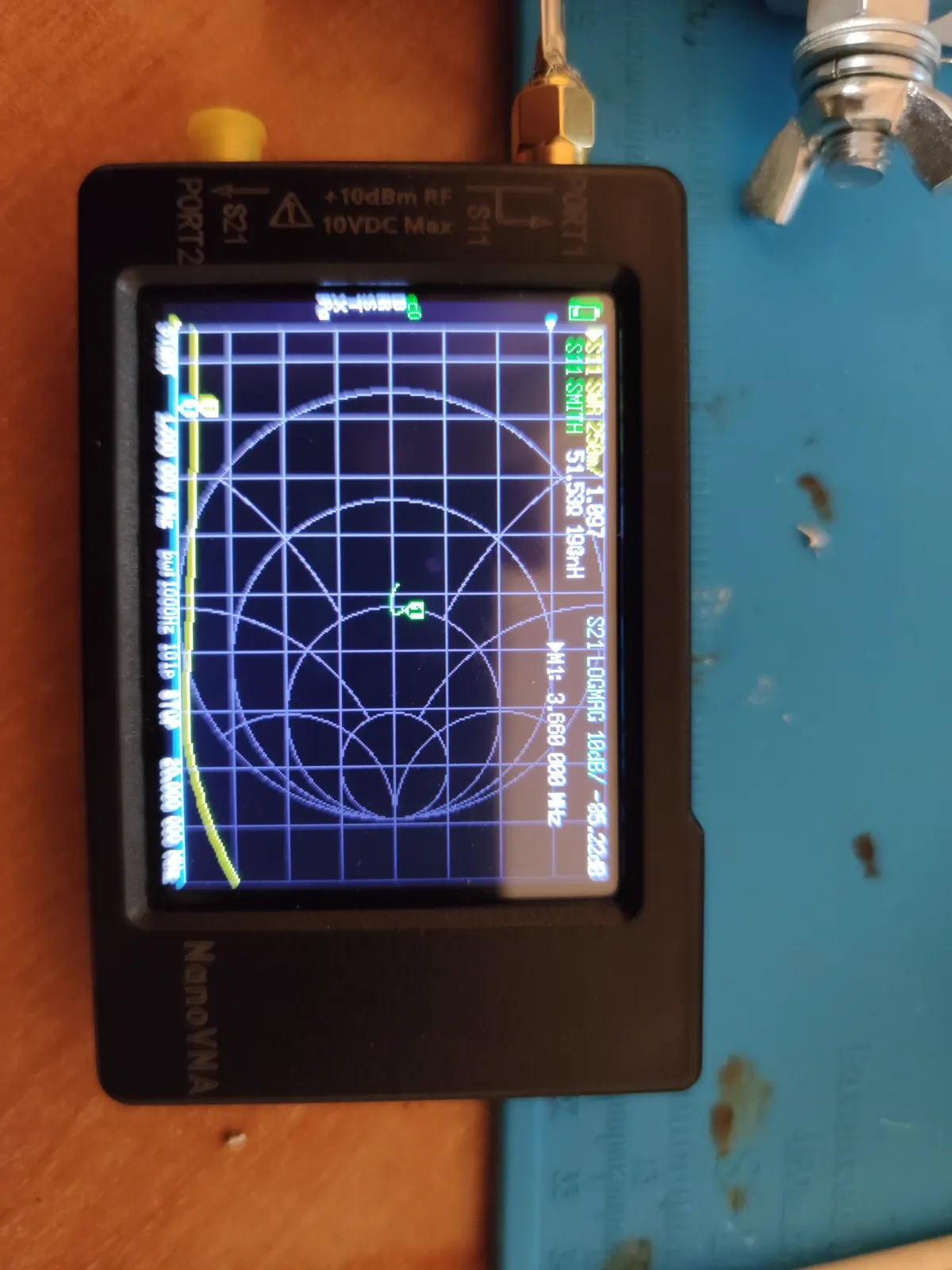
At 3.660 MHz: 51.5 Ω with 198 nH in series, SWR 1.097. Four and a half ohms of reactance against fifty of resistance.

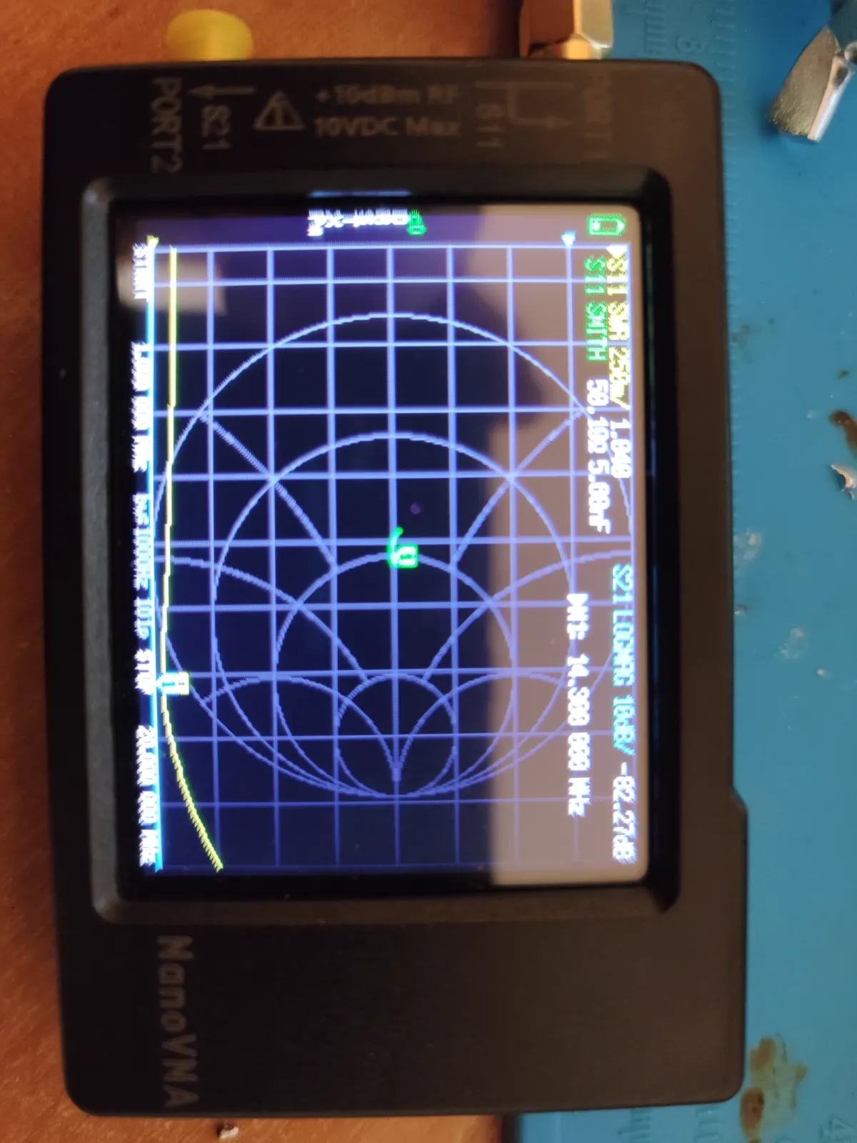
At 14.300 MHz: 50.19 Ω, SWR 1.040. Practically a perfect fifty ohms.

So from 80 to 20 metres the assembly stays transparent: it introduces neither loss nor a shift in impedance that would show at this scale.

And here is the point

This measurement is not a test of the balun as a balun.

I fed a signal into the cable side and looked at what the instrument saw. It saw fifty ohms. But it would have shown the same fifty ohms had I connected that same resistor through a length of cable — no ferrite required. S11 into 50 Ω measures the differential path: whether the transformer has eaten the match, whether it has losses or stray resonances in the working range. That question has been answered, and the answer is good.

The question a balun is fitted for in the first place — how much impedance it presents to common-mode current — this measurement does not touch at all. Common-mode current flows on the outside of the braid, that is, on the very conductor that does not exist in the S11 setup.

This is not an error of the instrument, nor of the method. It is an error of interpretation, and I made it: I saw an SWR of 1.04 and decided the assembly had been checked. Half of it had.

How to measure it properly

The common-mode impedance of a choke is measured differently: the two leads on one side are shorted together, the two on the other side likewise, and the impedance between those two points is measured. That is what common-mode current sees on its way. On HF the benchmark is a few kilohms across the working range; less means the braid is still acting as an antenna, just slightly worse at it.

It is done with the same NanoVNA and the same pair of hands. The only difference is where the leads go — and whether you have asked yourself the right question.

What can no longer be found out

The right measurement — common-mode impedance between the shorted pairs — was never made, and can no longer be made: the assembly is not available for it. The three or four kilohms in the table above remain a calculation from an equivalent material's data. A well-founded calculation, but not a measurement.

The box with its toroid did its job honestly: first quiet reception, later the first digital contacts. The one thing left undone was a single measurement — precisely the one the instrument had been taken out for.

And that is probably the thing worth taking from this note. The instrument was in hand, the assembly on the bench, time was unlimited. Only one thing was missing: the right question. Next time the list of what to measure gets written before the leads touch the terminals.